1. Introduction

A decision tree is one of the most traditional decision-making algorithms (e.g. MLP, SVM). With the growth of computing power (represented as GPU), the neural network with excessively deep layers has emerged, showing outstanding performance in a variety of tasks (e.g. computer vision, natural language processing).

However, the neural network’s excessively deep layers make itself a black box, hence causing its uninterpretable characteristic. This black box property brings the tree algorithm back to the fore since the tree algorithm has strength in interpretability with its transparency.

There have been several trials to enhance the performance of the tree algorithm by merging multiple decision trees (ensemble), modifying the structure of trees (cascaded tree), and combining with the neural network (neural-backed decision tree). This literature contains from the most traditional to the up-to-date tree algorithms with their suitable category of datasets (e.g. Tabular, Image data).

2. General Tree Building Algorithm

Traditional Decision Tree Classifier / Regressor

A decision tree is a data-driven decision-making algorithm, so its learning process also heavily relies on the distribution of the training data. At each level of the tree, the group of data (node) is split using a set of criteria. The most common criterion for splitting the tree are Gini impurity and Entropy.

Classification

Gini impurity is calculated as . For example, when the node is pure, the Gini impurity is calculated as, . Otherwise, when the node is composed of equally distributed two classes, the Gini impurity is .

Entropy is the measure of disorder, and is calculated as . When the node is pure, the entropy is calculated as . Otherwise, when the node is composed of equally distributed two classes, the entropy is .

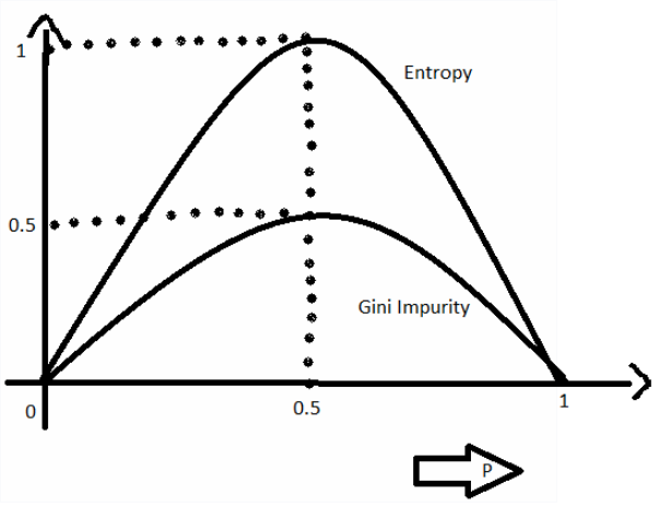
https://www.geeksforgeeks.org/gini-impurity-and-entropy-in-decision-tree-ml

As the above figure shows, we can see that Entropy is roughly proportional to Gini impurity. Entropy is the measure of disorder, so the purer node has lower entropy and Gini impurity. The decision tree classifier finds a split that minimizes Gini impurity or Entropy.

Regression

In the case of a regression tree, the tree finds a split that minimizes RSS (residual sum of squares) of the child nodes. However, from now on, we are going to discuss classification tasks for simplicity.

Ensemble

When multiple trees collaborate to make a decision, we call this methodology an "Ensemble Tree". Ensemble tree consists of "weak learners" or "base learners" (often called a "stump"). Bagging and boosting are the most popular ensemble tree algorithms.

Bagging

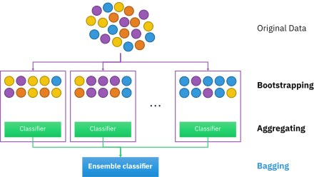
https://en.wikipedia.org/wiki/Bootstrap_aggregating

Bootstrap aggregating (Bagging) is the ensemble learning method to reduce the effect of the dataset’s noise. The bagging method builds multiple parallel classifiers for the subsets of the original dataset and averages the result of each classifier for the final result. One of the most powerful and popular bagging methods is a Random Forest algorithm. The number of features, maximum level of the tree, number of trees composing the forest are the hyperparameters used for the random forest.

Boosting

Boosting is an ensemble technique that combines classifiers in series to generate stronger classifiers from the sequentially connected weak learners. The figure shows how weak learners evolve by weighting the data.

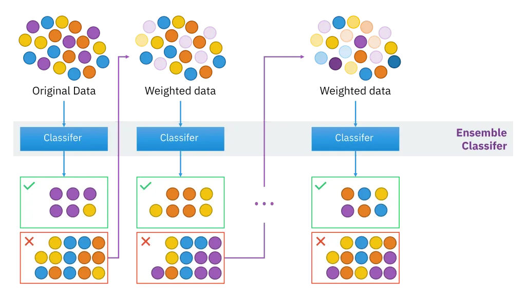
https://corporatefinanceinstitute.com/resources/knowledge/other/boosting

In detail, the ensemble output is a weighted sum of each weak learners.

• Each tree is created iteratively
• The tree's output is given a weight relative to its accuracy
• The ensemble output is weighted sum
• After each iteration each data sample is given a weight based on its misclassification
  • The more often a data sample is misclassified, the more important it becomes
• The goal is to minimize an objective function

is the loss function — the distance between the truth and the prediction of th sample

is the regularization function — it penalized the complexity of the th tree

The most popular boosting tree models are Gradient Boosting (which uses gradient descent to generate new learners) and XGBoost (regulation term added to gradient boosting) models. Especially, XGBoost outperforms state-of-art machine learning techniques in specific domains such as tabular data.

3. Backpropagation in Decision Tree

Oblique Decision Tree

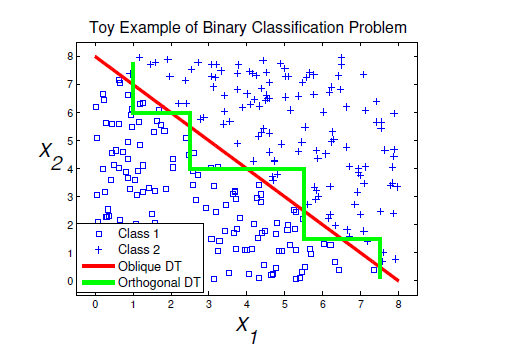
https://sites.google.com/site/zhangleuestc/incremental-oblique-random-forest

Unlike the traditional decision tree, which splits the node based on the value of a single feature, oblique decision tree sets the criterion as a linear (or nonlinear) combination of different features. As a result, the DoF (Degree of Freedom) of decision boundary increases and it enables clear classification with less level of the tree. However, the combination of features could make the oblique decision tree model less interpretable compared to the original decision tree.

Probabilistic Decision Tree (Soft Decision Tree)

The traditional decision tree is a deterministic decision tree; the sample passes through different levels of tree and is determined to a single final leaf node.

However, the probabilistic decision tree makes a probabilistic decision at the final leaf node by passing through a stochastic routing. In other words, the classifier doesn’t definitively give a single answer and gives probability of the sample’s class. i.e. All the samples reside in leaves probabilistically.

There are many preceding works on this, including "Fuzzy Decision Tree", Suarez et al, "Deep Neural Decision Forest (DNDF)", Kontschieder et al. We are going to cover how to DNDF is modeled and optimized, in the next section.

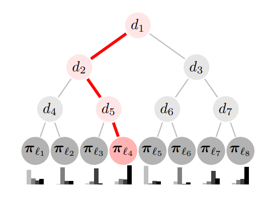
figure 1. https://www.ijcai.org/Proceedings/16/Papers/628.pdf

This method has several advantages over the deterministic model.

First, probabilistic model has high tolerance against the model’s mistake especially in the early stage. i.e. more stable. Unlike the deterministic model, probabilistic model can compensate the wrong choice in the early stage by the later stage because the final leaf node probability is calculated by the multiplication of each node’s probability distribution.

Secondly, by making the tree’s output continuous and differentiable, probabilistic model enables it to apply backpropagation learning process on the tree algorithm.

Backpropagation

This section cover how DNDF is constructed and optimized. Two major components of the model is internal node (split criterion, and leaf node (class distribution, ). DNDF is a full binary tree w/ all the leaves having same depth. Unlike the classic tree models in which each leaf has different depth, DNDF's leaves have fixed depth. All example data are passed down to the leaves, and decisions are made at leaf. Detailed explanation of the components are as below.

• : Categorical distribution (of the classes) that each leaves holds. Softmax is used.
  • Preceding work in Suarez et al. [1] simply use histogram as probability mass estimation
• : class 's value of
  • Arrowed value below is a single value . The value of softmax of class of leaf

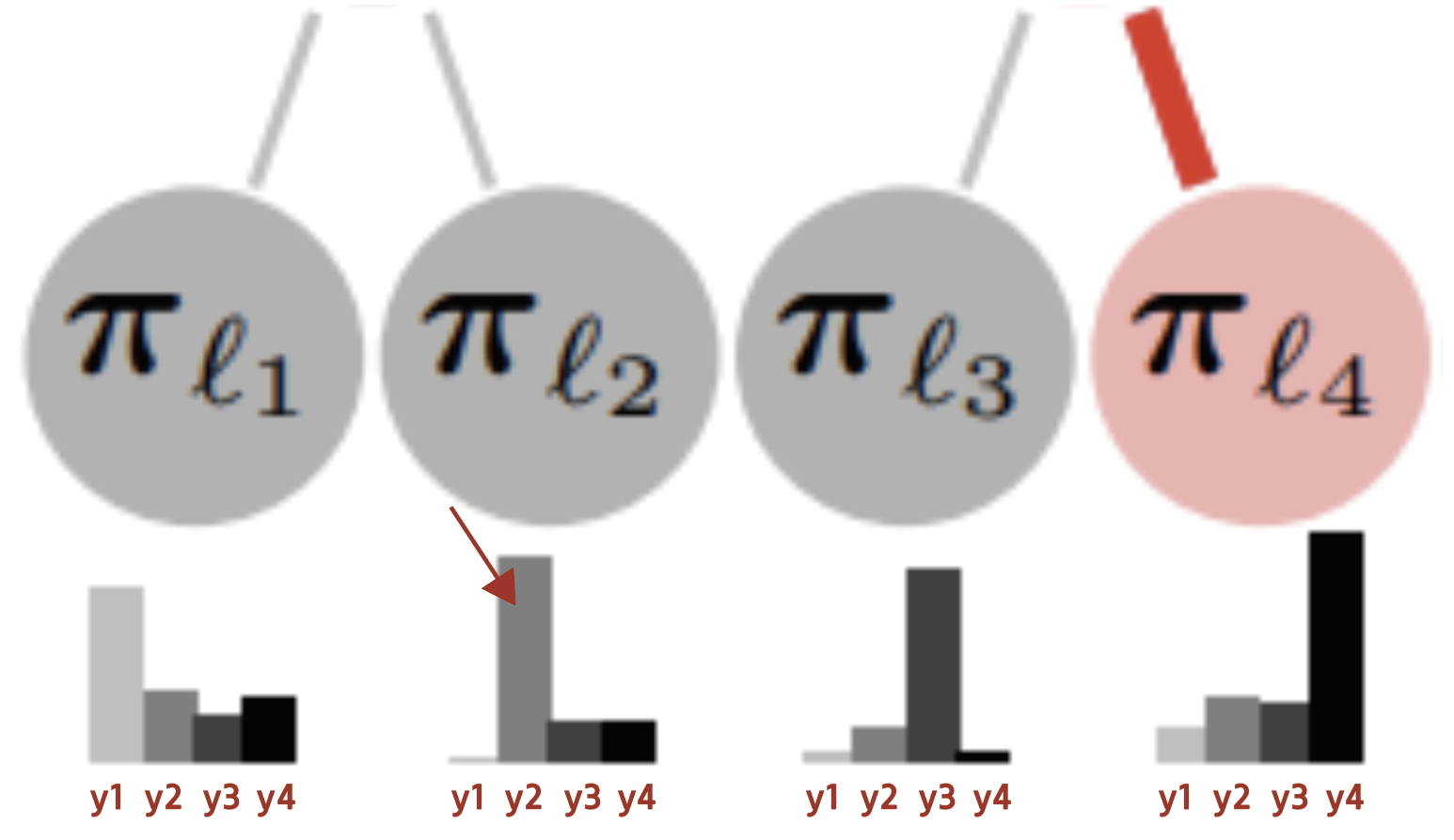
figure 2. say we want to update arrowed value, we update

• : Decision function(soft split criterion) that th node holds
  • Might be thought of as bernoulli random variable, modeled as a linear function of , that is discretized by sigmoid function
  • By setting as independent , it becomes similar to oblique decision tree. Here, it's shared throughout the model.
• : The final probability that sample will reach th leaf
  • e.g. following the path from the figure 1, we get
• : The final prediction, incorporating the entire leaves
  • Just think of it as mixture of softmaxes

Overall algorithm

1. Initialize and

   1. with unifrom prior, with some random distribution

2. For N epochs, run optimization below

   1. Estimation of by iterative method

      Iteratively update by full batch data, for enough steps(about 20steps in the paper) until convergence. Below is a single update of a single value of .

      is normalizing term, is the full batch training data, is the true target, is class 's probability in leaf , is indicator function.
      
      Say we're updating in figure 2. Again, the specific probability value of of . Let's look at the summation on righthand. Iterating the training data, if sampled , then , else if then .
      Reinterpreting, among the all training data, if those whose class equals to the updating class , then it's chosen and added to summation. Since denominator includes , every iteration adjusts the distribution w.r.t the contribution of to the entire leaves.
      
      Proof that gets better is in the supplementary of [2]
      
      p.s. Those who are familiar with Expectation Maximization(EM algorithm), refer to EM algorithm of multinoulli distribution.

   2. Update with SGD for mini-batch

      With negative likelihood loss,

      Run the typical optimization process,

      is the learning rate

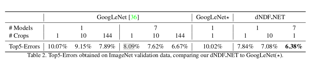
The paper shows better result of adding DNDF as the discriminant of GoogLeNet (dNDF.NET).

GoogLenet is a distributed implementation of the original GoogLeNet, and dNDF.NET replaces the softmax layer from the original ones.

"Globally Optimal Fuzzy Decision Trees for Classification and Regression", Suarez et al. [1]

"Deep Neural Decision Forest", Kontschieder et al. [2]

4. Advanced tree algorithm for tabular (low-dimensional) data: Cascading Decision Tree

Cascading Decision Tree

Cascading is a particular case of ensemble learning based on the concatenation of several classifiers, using all information collected from the output from a given classifier as additional information for the next classifier in the cascade. Unlike voting or stacking ensembles, which are multiexpert systems, cascading is a multistage one.

https://en.wikipedia.org/wiki/Cascading_classifiers

Learning tree model with modern datasets generates a large tree, which generates decision paths of excessive depth, making it hard to understand the tree's decision path.

"Succinct Explanations With Cascading Decision Trees (CDT)", Zhang et al. has suggested a way to overcome this problem, by separating the notion of a "decision path" and an "explanation path". Their main contribution was to shorten the explanation path to provide maximum interpretability of the model by stacking multiple stumps.

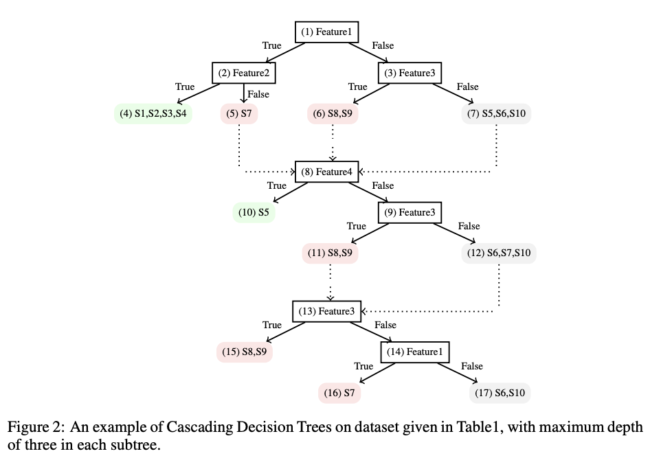
Compared to the comprehensive tree models, the CDT showed lower average depth of tree and thereby better interpretability.

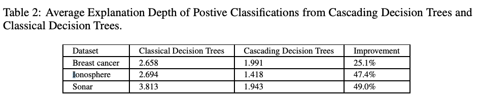
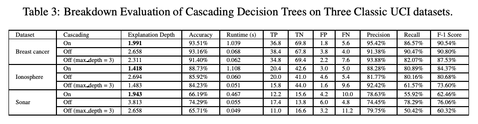
In addition to the improvement in interpretability, CDT also outperforms other tree algorithms in terms of accuracy with the tabular datasets.

Deep Forest

The "Deep Forest", Zhou et al. is motivated by the deep neural network’s deep layer property. It was intrigued by the insight that deep learning’s success owes to its layer-by-layer processing and its feature extraction ability.

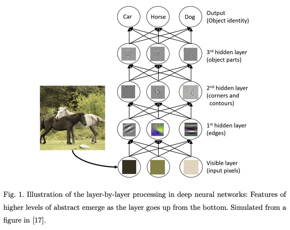
To utilize deep learning's feature extraction ability, Deep Forest has proposed "gcForest" (multi-Grained Cascade Forest). Each level is ensemble of tree forests (ensemble of ensemble) and it consists of different types of forests to encourage "diversity". The blue forests are completely-random forests, generated by randomly selecting a feature for split, growing until the leaf is pure. The black forests are normal random forests.

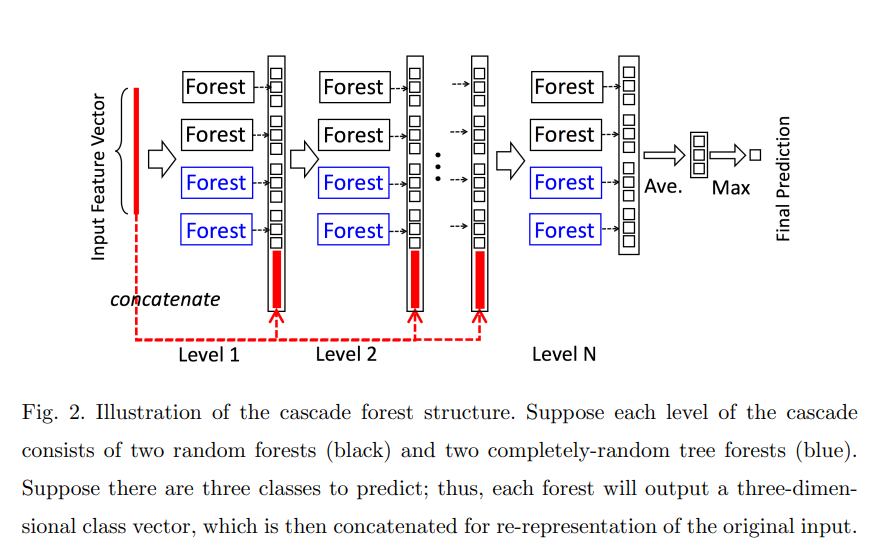
gcForest connects those random forests in series and use each forests’ output as the input to the next layer of random forests. And input dataset is processed with multi-grained scanning, producing different granularities of data and is concatenated to the input of each layer of the forests. The proposed scanning method uses sliding window to capture spatial/sequential relationships, so it can be used to encode image data or sequential data (see the paper for details of scanning method).

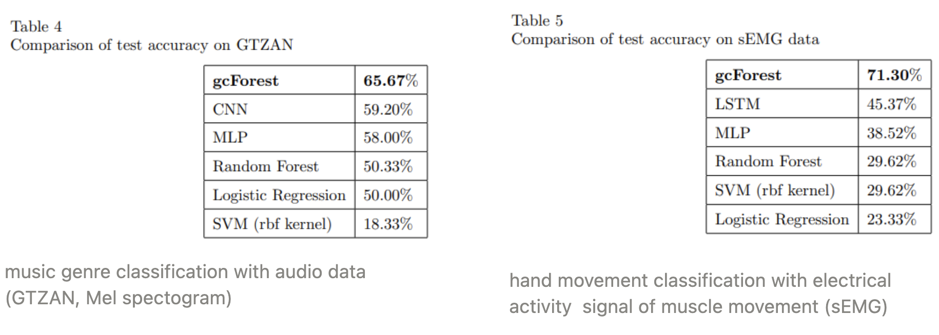
gcForest outperforms other machine learning techniques including conventional decision tree and neural network in some low-dimension datasets (e.g. IMDB, MNIST). However, for high dimensional data (CIFAR-10), deep neural network models outperforms. For time-series data (GTZAN, sEMG), it showed quite remarkable results.

5. Advanced tree algorithm for image (high-dimensional) data: Neural-Backed Decision Tree

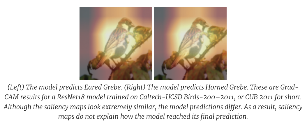
"Neural-Backed Decision Tree (NBDT)", Wan et al., is a hybrid algorithm which has replaced the final layer of the neural network with the decision tree in order to enhance the interpretability of a neural network model. While deep neural networks show great performance in image classification tasks, their deep and complex structures make them almost a black-box. There have been some trials to make neural networks interpretable: saliency maps such as GradCam. However, the saliency map only gives information about ‘which’ area the model is focusing, not ‘why’ the model is making a specific decision.

https://bair.berkeley.edu/blog/2020/04/23/decisions/

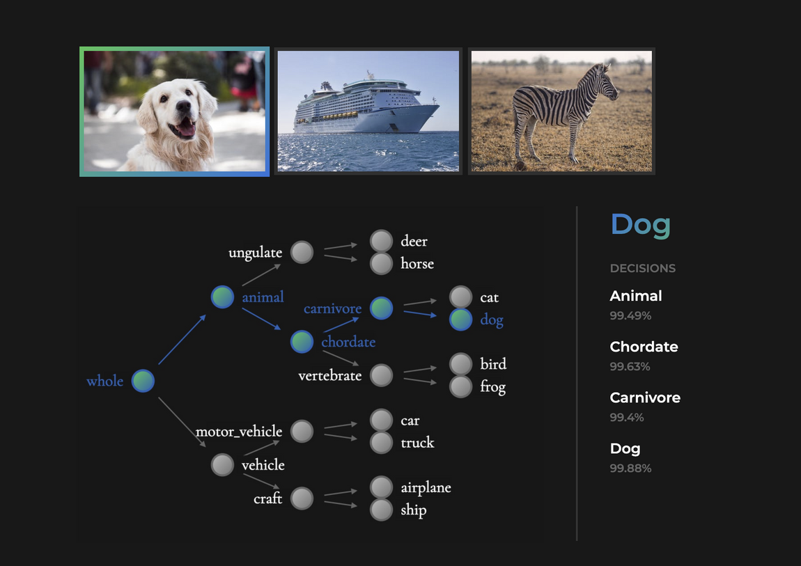
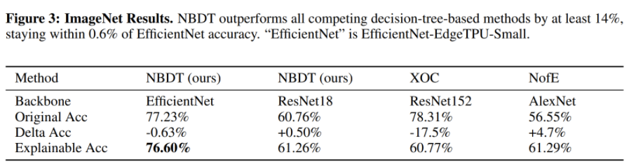
In contrast, the NBDT shows the full decision process by providing taxonomoical assignment to each node with negligible sacrifice in accuracy.

https://bair.berkeley.edu/blog/2020/04/23/decisions/

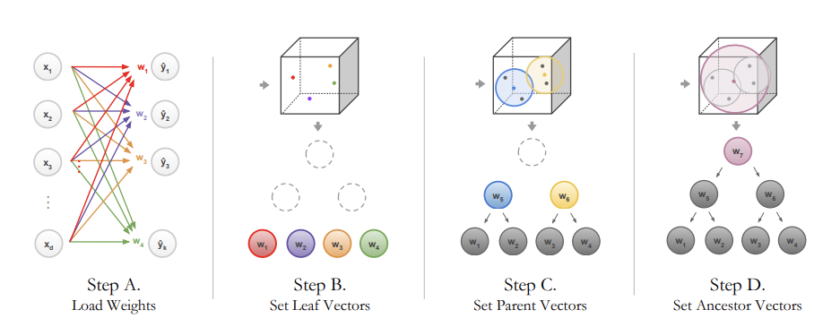
By unraveling the final layer of a pretrained neural network model, NBDT targeted both accuracy and interpretability. In detail, the NBDT has assigned the weight vector of the neural net’s final linear layer to the terminal node (leaf) of the decision tree. Taxonomically close classes are located closely in the leaf of the tree, so that their common parent node could have taxonomical meaning.

The tree is built bottom-up, calculating the parent node’s weight value by averaging weight values of its two child nodes. The inference made by the decision tree is probabilistic (soft decision tree).

NBDT starts from the pretrained neural network as the backbone structure and fine-tune the unraveled decision tree and pretrained neural network for better accuracy.

The loss function is given as

The cross entropy coefficient for the neural network decreases from 1 to 0 while the coefficient for the decision tree gradually increases. As a result, the model could preserve the feature extraction property of a neural network and build a precise tree model.

As a result, the NBDT shows an accuracy comparable to a neural network while showing much clearer interpretability according to their survey. In summary, NBDT has provided a new perspective about the tree algorithm by suggesting a weight-space-based tree, and not the feature-based tree.

6. Conclusion

High-stakes industries such as biology(or healthcare), finance, etc. still have high demands in decision trees because, decisions made from black-box are often unacceptable in the business. As a result, many services are yet being served with large, costly tree models, despite the success of of neural network.

For example, model for cancer prediction trained with genome sequence data (a single datum can take up to several gigabytes), model for credit scoring trained with huge demographics, are actively accepted models we can find in the real-life business.

So rather than discarding the models already trained with huge costs, one might think of an applicable situation for example, utilize pre-trained tree models and enhance their representational capacities with neural network. Then we might find a hybrid gray-box model that's more practical at the expense of, maybe a little decreased accuracy, but much more of an acceptable decision maker. The hybrid models often achieves even better accuracy as the algorithms introduced in this post exhibit.

Reference

• Deep Forest, Zhou et al.
  https://arxiv.org/pdf/1702.08835.pdf
• Neural backed decision tree, Wan et al.
  https://arxiv.org/abs/2004.00221
• Cascading Decision Tree, Zhang et al.
  https://arxiv.org/pdf/2010.06631.pdf
• https://indico.fnal.gov/event/15356/contributions/31377/attachments/19671/24560/DecisionTrees.pdf
• https://arifromadhan19.medium.com/regrssion-in-decision-tree-a-step-by-step-cart-classification-and-regression-tree-196c6ac9711e