1. Introduction

This post aims to introduce the integration of graph database (GraphDB) and deep model based Machine Learning (ML) on a graph. While this has not caught a wide audience yet, we believe this can be one of the successful applications of Machine Learning. Like improvement in ML opened the promising field of optimizing Relational Database System (RDBS) using ML, we expect the improvement of Machine Learning on a graph can shed a new light on the optimization of GraphDB.

📌 Integration of database and machine learning in RDBS

Here we show the example how ML can be helpful in enhancing the optimization of RDBS.

The order of "JOIN" operations in SQL can significantly change the overall performance. Therefore, determining the order of "JOIN" operations is one of the important tasks to optimize the RDBS operations. In 2018, UC Berkeley Rise Lab introduced optimizing the order of "JOIN" queries using Reinforcement Learning.

Classical algorithms solve this problem by dynamic programming (DP). For instance, assume we have three tables in the database, which are S (Salary), E (Employee), and T (Taxes), and want to perform the query below.

SELECT SUM(S.salary * T.rate)
FROM Employees as E, Salaries as S, Taxes as T
WHERE E.position = S.position AND
              T.country = S.country AND
              E.position = ‘Manager 1

This query requires RDBS to join three tables, {E}, {S}, and {T}. To solve the optimal cost of "JOIN
" operation for two tables, we can formulate the below recursive equation:

Therefore, we first save , which is just time scanning each table, and then define using above recursive equation. Then, we finally define by findning minimum from.

This problem can be solved using DP. When we have sufficient memory, DP is a powerful way to find optimal in a recursive equation. However, when it is hard to save all possible operations in a table, Reinforcement Learning (RL) can be one of the alternatives for DP, by constructing a neural network that can approximate operation tables. We omit the detailed approaches for executing "JOIN" operation using RL, and link the paper and blog posts instead.

This shows that ML can be one of the promising approaches to optimize an operation of a database. We believe MLs and deep models are not only applicable to RDBS, but also in the field of GraphDB, with the recent progress in GraphDBs and GNNs.

📌 Content of the article

The content of this post is organized like the following. First, we explain what a graph is, and what a GraphDB is with a few well-known GraphDB libraries. Second, we introduce the field of Graph Neural Network (GNN), one of the ways to efficiently perform a deep model on a graph, and a couple of well-known libraries for GNN. Third, we summarize tasks in GraphDB, introduce how classical algorithms solve those problems, and analyze how deep models on a graph can be efficient for those tasks. Finally, we observe what are the future research challenges in this field.

The aim of this article is to overview previous studies and possible research directions of utilizing deep moels and GNNs for GraphDB, instead of explaining each algorithm in detail. Therefore, instead of delving into the specifics of algorithms and theories, we will point out key ideas and refer to well-written references for the details.

2. Graph and GraphDB

📌 Graph

A graph is an object that aims to illustrate the relationships among entities. In a mathematical language, a graph can be defined as a tuple G = (V,E), where V is a vertex set and E is an edge set. But in various domains more specific definitions, rather than this general one, are more useful. Based on how to define the vertices and the edges, there are many types of graph representations, one of which is a simple undirected unweighted graph. We can have more complicated graph representations by appending weights, directions, node properties, and edge properties as needed.

📌 GraphDB

A relational database can represent a graph using a table schema. But graphs usually do not fit well into such a representation, and therefore classical relational databases often fail to process graph data in an efficient manner. Graph Database (GraphDB) aims to enhance the performance of storing, processing, and managing graph datasets, by implementing a graph-specific database.

Graph Storing methods in GraphDB

A GraphDB needs to store nodes, edges, and properties in a efficient manner.

Nodes and properties are usually stored in a vector, and edges are usually stored in an adjacency matrix or adjacency list, with each relationship as an element of the list or matrix.

While a matrix representation has advantages in indexing and referencing, a list representation has the benefits of saving memory spaces. Many GraphDBs prefer to choose the list representation due to the limit of the memory capacity, but each has a different implementation.

Libraries

According to the https://db-engines.com/en/ranking/graph+dbms, Neo4j and JanusGraph are the GraphDBs that are widely used in April, 2021. We briefly introduce how these t GraphDBs differ.

• Neo4j

Neo4j is a Java and Scala-based GraphDB, and it is currently the most widely used GraphDB. Neo4j stores graph data using the variation of an adjacency list. In Neo4j, each node has a pointer to the first relationship. Then, a doubly-linked list of relationships follows after this first relationship. This enables Neo4j to store multiple relationships.

Like there is a query language SQL for RDBS, Neo4j also has its own query language, called Cypher. We can interact with Neo4j Database using Cypher. Cypher has an advantage in code readability, while it suffers the lack of optimization possibilities.

• JanusGraph

JanusGraph is an open-source Java-based GraphDB. JanusGRaph stores data using adjacency lists. It maintains the adjacency list of each vertex in sort order with the order being defined by the sort key and sort order the edge labels. The sort order enables efficient retrievals of subsets of the adjacency list. The below shows a brief structure of an adjacency list in JanusGraph. Each property contains what property it is with the key. And each edge contains what relationship it is and what is adjacent vertices.

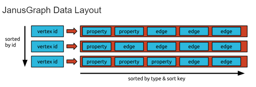
JanusGraph Internal. Reference: https://docs.janusgraph.org/advanced-topics/data-model/

This adjacency list is stored by Bigtable data model, which is a wide column storing table. Each vertex is a key, and each adjacency list is a value. Since JanusGraph uses a Bigtable, Janusgraph has a freedom in storage backends if the storage backend supports the JanusGraph. The possible candidates of storage backends for JanusGraph includes Apache Cassandra, Apache HBase, and Oracle Berkeley DB Java Edition.

JanusGraph recommends Gremlin query language for interactions. Gremlin has the advantage of very compact syntax and higher optimization level compared to Cypher, but it lacks code readability compared to Cypher.

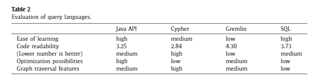
Comparison between query languages. Reference: Querying a graph database – language selection and performance considerations

3. GNN

A graph neural network (GNN) takes graph data as an input and implement Neural Network architectures in a graph-specific way.

📌 Representation learning and GNN

GNN is closely related to representation learning, whose goal is representing raw input data in a more "meaningful" way, that is, encoding the input data to some particular embedding that enables to extract information more easily.

When we use NN architectures, we regard the space of vectors before passing the final layer as a "representation". The final layer works as aggregating the representation to solve the given task. This point of view is applicable to all NN-based architectures. The field of obtaining meaningful representation for the task, especially using ML, is called "Representation Learning".

To use ML-based approaches, GNN tries to learn the "good representation" of the graph, and use this representation to solve the given problem. Therefore, the performance of a GNN is closely related to the quality of the representation. Typical representation learning tries to embed data into Euclidean space, but it does not have to be a Euclidean or even a metric space.

📌 GNN architectures

Implementing Neural Network Operations in Graph Domain

Inspired from recent progresses in Computer Vision (CV) and Natural Language Processing (NLP), there were attempts to integrate the architectures that successfully worked in those domains, such as Convolutional Neural Network (CNN) and Attention Network, with graph-theoretical approaches. With some attempts, It revealed that a "message-passing" scheme in a graph theory fits well with the NN architectures. As a result, many architectures are developed based on the message-passing scheme.

In the following sections, we first introduce the message-passing scheme, and review some widely-known GNN architectures, Graph Convolutional Network (GCN), Graph Attention Network (GAT), and GraphSAGE, which are based on the message-passing. There are more algorithms developed recently, for example, Graph Neural Tangent Kernel and Graph Wavelet Convolutional Network, but we omit those works for this article.

Message-Passing Scheme: A general framework of GNNs

One of the fundamental approaches to interpret the various graph algorithms is Message-Passing, a theoretical framework that views each graph node containing a message and analyzes how these messages are passed through their neighborhood. This implies that we can calculate backward from the neighbors to retrieve the original node. In other words, aggregating the message from neighbor nodes can reconstruct the message of the original node. This consists of 3 steps.

1. Computation of neighbor's messages
   • First, we need to compute the message between our original node and neighbor nodes.
   • For a node and one of its neighbor nodes , we denote current representations with th update of and as , and the current relationship between these two representations as .
   • For the initial step ( , we set and edge .
   • Then, by pre-defined message computation function , we compute a message between and as .
2. Aggregation of messages
   • Now, we aggregate all messages of neight nodes computed in 1.
   • With a pre-defined aggregation function , we aggregate messages of , a set of neighbor nodes of .
   • With a slight abuse of notation, an aggregated message for would be
   • This aggregated message can be interpreted as information of the node reconstructed by .
3. Updating the representation with the aggregated messages
   • Lastly, we update a representation using pre-defined update function by
   • This means that we update representation based on current representation and neighborhood messages obtained in current representation.

The underlying idea of message-passing is intuitive but powerful. It gives us a theoretical justification for capturing structural information of the graph via iterative methods.

Graph Convolutional Network (GCN)

GCN is a most widely known way to implement a CNN in graph domain. It has its theoretical background in graph spectral theory. We omit the theoretical backgrounds of GCN and refer this well-written blog post (Korean) for detailed theoretical explanations. Instead, we propose general steps of GCN, and explain key ideas.

While the original GCN paper did not denote their procedures in this message passing viewpoint, it is easy to check if we set the as a linear function using weights and degree normalization, as a sum, and as an activation function, then procedure 1~3 becomes a GCN layer. We describe the procedure in details for th iteration.

1. Computation of the messages
   • We set a linear function as follows: , where is a linear matrix. In this case, we consider the relationship . The is a parameter of Neural Network and will be trained.
2. Aggregation of the messages
   • By defining as a sum of all neighbors with adding the own node to its neighbor, we can calculate the aggregation .
3. Updating the representation with the aggregated messages
   • We define the function as the activation function . Then, the final architecture would be

We can easily check that this message-passing scheme corresponds to expressing the original formulation of GCN as follows,

where where is an adjacency matrix, and is a diagonal node degree of . This enables us to interpret the GCN network as the following message-passing scheme: each GCN layer aggregates 1st hops of current nodes, therefore th GCN layer is an aggregation of message till th-hop information. This interpretation works well for experimental results: unlike general NNs that usually perform better with deeper layers (if we ignore overfitting), GCN tends to perform worse when we append more layers. Appending too many layers means aggregating too many hops, and it can lead to diluting the information from nearby hops.

Graph Attention Network (GAT)

GAT is an architecture that is inspired from both GCN and Attention network, which is a widely used architecture in NLP. GAT also follows the message-passing scheme. Meanwhile, GAT tries to be more flexible than GCN by making some part of its architecture more implicit. Like we did in GCN, we will review GAT from the viewpoint of the message-passing scheme.

1. Computation of the messages
   • GAT also takes the same formula with GCN, by setting as a linear function. However, while GCN has explicit normalizing constants defined by degrees, GAT makes this coefficient implicit, so that we can have more flexibility.
   • First, we define attention function by NN, where is a hyperparameter (pre-defined intermediate layer's dimension). The original paper proposes the attention function as a concatenation of two nodes and followed by a single-layer feedforward NN, written by . denotes the concatenation operation.
   • Then, we compute , and , where will act as a normalizing coefficient.
   • Then, the message is computed by
   • The fundamental difference between GCN and GAT lies in the coefficient. GCN has fixed coefficient structures for all nodes, whereas GAT can have different coefficient structures node by node by defining implicitly. It means that we can consider different weights, or attentions, of messages, and therefore able to handle more flexible structures.
2. Aggregation of the messages
   • The aggregation part of GAT is same with GCN, using a sum of the messages. It can be formulated as .
3. Updating the representation with the aggregated messages - The update part is also same, if we use a single-head attention. It can be written as - To stabilize the learning process, GAT can use a multi-head attention, i.e. multiple attention networks. To be specific, we construct attentions, and accordingly Then, we make an update by concatenating messages from multiple attentions.
   In this case, until final layers, and at the last layer .

As mentioned above, GAT can contain more information about the structures of the graph implicitly. Moreover, GAT has an advantage that calculating 's does not require an entire graph structure. Note that GCN's coefficients are constructed by degree information. It implies that we need to have degree information of all nodes "before" we actually conduct the algorithm. On the other hand, GAT's 's are derived from the network, so that the algorithm does not require us to have the information of the entire graph at the time of the computation.

This means GAT can learn the representation of the graph that is "inductive". In other words, GAT can learn the representation that can handle even "unobserved" nodes. If there is an unobserved node, GCN may not work as it intended as its degree information is likely to be incorrect. Meanwhile, GAT works without the degree information. and we expect attention networks to implicitly capture the information of unobserved nodes even if we are not able to observe such nodes. Simply put, even when we cannot observe a full graph we can use GAT to construct an ML model for the graph.

GraphSage

As mentioned in the GAT section, GCN is not capable of inductive learning, as it requires all degree information. GraphSAGE did not use this normalizing coefficient and modifies the aggregation function from "Aggregation of neighbors" to "Aggregation of samples of neighbors" (step 2 in message-passing). The sampling is to reduce the time complexity and the memory complexity, but it can also serve as a new viewpoint that unobserved nodes are just nodes that are not sampled.

📌 Libraries

Many GNNs use matrix operations for computations, so any libraries that support efficient matrix computations and gradient descent algorithms can conduct GNNs. Meanwhile, two well-known Python-based libraries exist, which are Pytorch-Geometric (PyG) and Deep-Graph-Library (DGL).

While both libraries provide similar features, a major difference between two is in their data representations. PyG represents data in Pytorch tensors. Therefore, it is more compatible with Pytorch than DGL. Meanwhile, DGL's data interface follows NetworkX, which is a widely used Python graph library. Therefore, DGL has an advantage in processing raw graph data using NetworkX. The choice of the library depends on whether you want a compatibility for raw data or the training process.

4. GraphDB tasks, classical algorithms, and deep model based approaches

All databases try to reduce time and memory complexity and at the same time perform various querying algorithms accurately, and GraphDB is not an exception. Time-complexity for GraphDB is essential when algorithms require more than . The number of edges in a graph can be at maximum , and therefore many graph algorithms suffer from time complexity when or more. Also, many classical algorithms are based on linear models, which prohibits algorithms to encode rich data-driven information. One way to overcome these obstacles is using deep ML models for the graph domain. This may increase performances, enable algorithms to encode data-driven information, or both.

Among deep models on a graph, GNNs are especially powerful when detecting the overall structures of the graph. Message passing enables GNNs to aggregate neighborhood information into the node without fully exploring exponential search space. (need reference) Therefore, GNNs may shed light on graph algorithms that are related to the global structures of the graph. There are also other deep models that do not use GNNs and instead use their own approaches to efficiently encode the information of the graph. We observe deep models based on both GNNs and not comprehensively.

GraphDBs implement many graph algorithms. The list of algorithms needed for GraphDB is mentioned in https://neo4j.com/developer/graph-data-science/graph-algorithms/. In the listed algorithms, this article focuses on the tasks of node similarity, link prediction, centrality, and community detection. While there exist many classical algorithms that work well for the tasks, they are based on heuristics. Replacing those algorithms with data-driven ones is an active field of research, and using a deep model is one possible approach. In this section, we introduce baseline classical algorithms and deep model based approaches, including approaches using GNN, for each algorithm.

📌 Node similarity

Node similarity algorithms are one of the most used algorithms in GraphDBs. For example, when using a node similarity algorithm for a recommendation system, we first set a threshold . Then, for a given node , recommended nodes are defined as follow: . In this case, the similarity metric between two nodes determines the quality and the performance of the recommendation. Therefore, it is important to define a "good" similarity metric.

Classical algorithms

Here we review two criteria to define the node similarity. The first is the proximity between the nodes. This is more intuitive, based on the idea that similar nodes tend to gather as a community. This concept is also noted as network homophily. The proximity is usually measured by the number of hops, instead of the distance itself. The reason hops are more widely used than the distance is that hops determine the similarity of the node information. When we think of a message passed by the node, the more hops the message percolate, the more diluted the message. Therefore, nodes with fewer hops, not the closer distances, share similar messages, or information.

The second is to define a similarity based on node roles. For this criterion, we need to define when two nodes have same role, or in other words, when two nodes are equivalent. Widely known equivalence relations between two nodes are structural equivalence, automorphic equivalence, and regular equivalence.

• Structural equivalence regards two nodes as equivalent if they share same neighborhood.
• Automorphic equivalence considers two nodes the same when interchanging two nodes does not change the graph structure.
• Lastly, when two nodes have the same neighborhood structure, while not necessarily share the same neighbor, they are called regular equivalent.

The relationship between these equivalence can be described as .

Once we defined the equivalence relation, we can measure "similarity" based on how much they are equivalent. Among those equivalences, structural equivalence is most widely used. In this article, we review one that is the most widely used similarity metric that is based on structural equivalence, the Jaccard similarity, which is based on the Jaccard distance.

Jaccard distance is a distance between two sets. For the two sets and , Jaccard Distance between and is defined as . We can inversely define Jaccard Similarity, by Intuitively, it compares how many set elements coincide.

Many GraphDBs define similarity of two nodes and using Jaccard Distance between neighborhoods of those nodes, and . In formula, . It means that similarity of two nodes are based on how similar their neighborhoods are.

Theoretically, Jaccard similarity's time complexity for n sets is quadratic complexity, . This complexity can be reduced using heuristics. For example, Neo4j reduces the complexity by ignoring disconnected nodes.

Beside Jaccard similarity, there are other similarity metrics to use.

• Algorithms that are based on structural equivalence are cosine similarity, euclidean similarity, and Degree Pearson Correlation Coefficient.
• RoleSim is an algorithm that tries to capture the similarity based on automorphism equivalence.
• For regular equivalence, there is an algorithm that resembles Katz centrality algorithm. We refer to this presentation for various similarity measures for each equivalence relationship.

While these classical methods are intuitive, they can only measure the similarity based on pre-defined equivalence relations. For example, if you choose to use the Jaccard Similarity, it means you ignore other types of equivalences. Moreover, these algorithms may ignore hidden edges that are not observed yet, by using deterministic algorithms.

For a detailed discussion of defining node similarity, we refer https://web.eecs.umich.edu/~dkoutra/tut/sdm14.html and https://en.wikipedia.org/wiki/Similarity_(network_science)

Graph Machine Learning based: similarity in embedding space using Node2Vec - a graph embedding algorithms

Creating an embedding is one of the ways to measure the similarity metric. Once the embedding of the graph is trained, we can use the metric of the embedding space as a similarity measure. In this case, the quality of the similarity metric would mainly depend on how the embedding space is trained.

If we have a specific task for calculating node similarity, for example, recommendations, then we can train the embedding that maximizes our task performance. Then, metric in the embedding space naturally become node similarity, that best fits with the task.

Otherwise, if we do not have a specific task but just want to embed the space and calculate the similarity, we build the embedding space that preserve the features of the graph. There are many ways to retrieve features of the graph. Here we review Node2Vec, the random walk based algorithms. For other algorithms, refer http://snap.stanford.edu/proj/embeddings-www/files/nrltutorial-part1-embeddings.pdf.

Node2Vec is an embedding algorithm that is inspired by the skip-gram architecture in Natural Language Processing (NLP). Node2Vec learns features of the graph in two steps. The first step is to convert graph data into "sentence-like" data by sampling strategy, and the second step is to conduct skip-gram architecture. For the details of the Node2Vec algorithm, we refer to the original paper and this blog post.

The first step is to convert graph data into "sentence-like" data, or in a language of graph theory a directed subgraph, by choosing a sampling algorithm that is based on a random walk, which provides a probabilistic way to interpolate Breath-First-Search (BFS) and Depth-First-Search (DFS). BFS focuses more on node-proximity-based similarity, while DFS focuses on node-role similarity, or more precisely, structural equivalence.

A random walk visits the neighborhood of the node based on each edge's probability. Then, the way to determine the probability of selecting each edge becomes the crucial part. Node2Vec proposes to use 2 hyperparameters to determine the probability of the edge.

• , the return parameter, controls revisit probability, and therefore can control how much we will focus on local information.
• On the other hand, , the In-Out parameter, controls the probability of exploration to new nodes. By , we can determine how much we will focus on global information.

In this way, Node2Vec accommodates both structural equivalence similarity metric and proximity-based similarity metric.

After the sampling algorithm is fixed, then for the and we define the neighborhood of generated by . Once the neighborhood is defined, we can extend the architecture to a skip-gram architecture that is used in Natural Language Processing (NLP).

Let our embedding function be . The objective function of Node2Vec is defined as a log-probability of reconstruction of neighborhood structure given feature embedding. In a mathematical form, it is written as the follow: .

Under the assumption of

• conditional independence between neighborhood nodes, and
• symmetry in feature space between a node and its neighborhood, the objective function becomes tractable, written by . The former part is hard to compute, so they are computed by negative sampling. We omit the detail and refer for Node2Vec papers for this part.

Therefore, overall procedures can be summarized as follow: first, you perform the random walk. Then, based on a random walk, you compute the log-likelihood based on skip-gram architecture. The second part is usually conducted by Word2Vec algorithm. Then, you use Stochasrtic Gradient Descent (SGD) to train the parameters. Below is the algorithm denoted in the Node2Vec paper, "node2vec: Scalable Feature Learning for Networks".

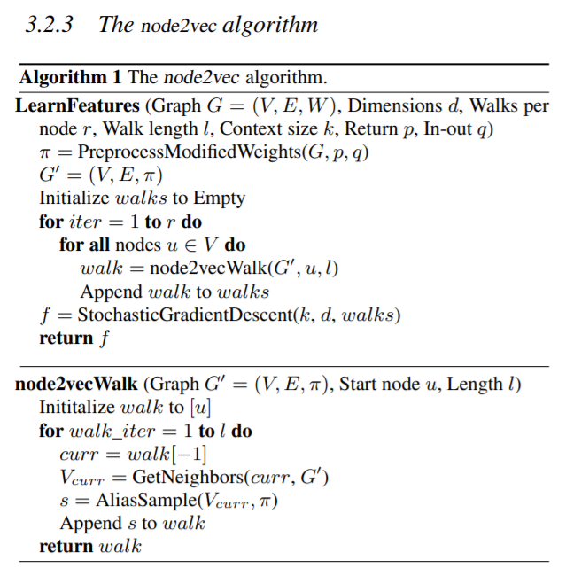
From node2vec: Scalable Feature Learning for Networks

📌 Link prediction

Link prediction is also one of the key tasks in recommendation and graph completion. The task is to determine the closeness of a pair of nodes. This task is closely linked to the node similarity task.

Classical algorithm

Link prediction tasks using classical algorithms are basically the same as defining which similarity metric to use. Most link prediction methods are measuring similarity based on Structural Equivalence. Theoretically, link prediction scores are the same with similarity scores, and we can use any similarity metrics, such as Jaccard Similarity, for predictions. However in practice, link prediction tasks use less rigorous but more simple scores, since we do not need the accurate similarity scores.

Therefore, Link prediction algorithms use heuristics to calculate the score that is similar to similarity metrics, with efficient computations. Existing link prediction algorithms can be categorized based on the maximum hop of neighbors needed to calculate the score. Common Neighborhood (CN) and Preferential Attachment (PA) are the first-order heuristics. CA score is defined as , and PA score is defined as . While they are the simplest way, they omit the normalization by the size or the type of neighbors as Jaccard did. To efficiently normalize without large computations, there are Resource Allocation (RA) and Adamic-Adar (AA), which is second-order heuristics. RA is calculated by , and AA is calculated by . By summing or , if sharing neighbor is universally connected, then be higher, and the score would be lower. Therefore, by this we can normalize the score by valuing the common neighbors that are uniquely connected each other more than that are universally connected with another nodes.

There are also more algorithms for link prediction tasks, including higher-order heuristics. We refer to Appendix A in SEAL paper (SEAL algorithm will be discussed in the below) for other algorithms.

Deep model & GNN based algorithms: WLNM and SEAL

Instead of defining the similarity metric and directly apply it for link prediction tasks, Deep model based algorithms try to capture structural and inherent information of the graph. We introduce two well-known algorithms in this section, WLNM (Weisfeiler-Lehman Neural Machine) and SEAL (Subgraphs, Embeddings and Attributes). WL is deep model that uses MLP, while SEAL is GNN-based model, as it uses GCN.

• WLNM

WLNM is inspired by the Weisfeiler-Lehman (WL) graph isomorphism test algorithm. WL tries to label nodes and figure out whether two graphs are labeled the same. To this end, WL test proceeds like a message passing scheme: 1) we initialize nodes with the same label, then 2) we aggregate neighbor nodes to update the current label. 3) This continues until node labels converge. The difference is in the initialization, the terminal conditions, the aggregation function and the update function. Naturally, WL algorithms consider structural features of the graph as the message passing scheme does.

Likewise, the WLNM algorithm captures structural information of the graph and uses this information to predict the link. WLNM consists of three steps. We illustrate these steps in the case of predicting a link between two nodes and .

1. Extracting sub-graphs
   • For a pre-defined parameter , we define -enclosing subgraph: Starting from , append neighborhood nodes, , of the set until .
2. Subgraph pattern encoding (Or, Node labeling and encoding)
   • Now, for the obtained subgraph in 1, we perform the modified WL algorithm, called a Palette-WL algorithm, to obtain node labeling (or coloring in a notation of the original paper). If there is a tie, the algorithm uses a Nauty algorithm, a graph canonization tool, to break the ties. We omit the detail of Nauty algorithm.
   • While classical WL algorithm can also perform the same task, Palette-WL modifies an aggregation function using hashing to label nodes fastly. We omit this part since it is not our interest.
   • After obtaining the sorted labels, or colors, the algorithm builds the adjacency matrix for the subgraph. Then, we set each column of the adjacency matrix as input vectors.
3. Neural Network Training
   • Since input (column of the enclosing subgraph's adjacency matrix) can be regarded as labeled data (1 if two nodes have connection, 0 otherwise), we can now view a problem as a classification task. Therefore, we train the Neural Network using the labeled data with Fully connected Multi-Layer Perception (MLP), classify the node, and conclude that output probability is the probability of link between these two nodes.
   • Note that WLNM uses fully connected MLP. While WLNM used a NN to predict the link, it is not, strictly speaking, using a GNN. WLNM just uses vectors, the column of adjacency matrix, as inputs, instead of using these "graphs" as NN inputs. It discards the information the graph contains, especially node features.

While the WLNM is more capable of incorporating various graph properties than similarity-based heuristics when predicting the link, the role of hyperparameters, especially the number of neighbors of the enclosing subgraph , may be crucial in the algorithm. Therefore, it depends on pre-defined variables as heuristics do. Moreover, the NN architecture used in WLNM discards information of the graph using MLP, as mentioned above.

• SEAL

SEAL is a variant of WLNM, in the sense that it also consists of the above 3 steps. However, SEAL modifies some details in those steps to better capture the node features and latent information. The major difference between SEAL and WLNM is that SEAL uses GCN instead of MLP, which enables it to preserve the information required for link prediction.

1. Extracting sub-graphs
   • Like WLNM does, SEAL also tries to capture the enclosing subgraph of the and . However, instead of using -enclosing subgraph proposed in WLNM, SEAL proposes to use -hops enclosing subgraph, which is the union of 1 ~ -hop neighbors of and .
2. Subgraph pattern encoding (Or, Node labeling and encoding)
   • Instead of using the WL labeling algorithm, SEAL proposes Double-Radius Node Labeling (DRNL). It is a label based on how far each node is from our target nodes and . For node , is labeled with higher number as the sum of distances from and , , goes larger.
   • Unlike WLNM which only considers the enclosing subgraph, SEAL tries to incorporate node features and latent information as well. Therefore, SEAL constructs enclosing subgraph's node feature matrix by the following procedures.
     1. First, we make one-hot encoding of the labels obtained above.
     2. Then, SEAL embeds the original graph (not the enclosing subgraph) and uses this embedding to consider latent information. When generating the embedding, the algorithm uses the trick called "negative injection", which is to add false negative edges. By this we can avoid GNN from overlooking non-existing edges. The embedding algorithm can be chosen from existing methods, such as Node2Vec or Graph Autoencoder.
     3. After obtaining the one-hot encoding of the labels and the graph embedding, we concatenate each node's one-hot encoding and embedding, and regard it as a "node feature vectors". We construct an enclosing subgraph's node feature matrix based on this node feature vectors.
3. Neural Network Training
   • After we obtained , the node feature matrix of the enclosing subgraph, and , the adjacency matrix of the enclosing subgraph, we can compute GNN using GCN network, which can both consider node features and the adjacency matrix. By this, we can have more richer information besides WL labels, such as latent information and adjacency matrix.

📌 Centrality

Centrality algorithms measure the importance of distinct nodes in the graph. Centrality algorithms are crucial in many graph tasks, such as search engines and recommendation systems.

Classical algorithms: PageRank and Betweenenss Centrality

Like node similarity tasks and link prediction tasks, classical centrality algorithms first need to define what centrality is. Among various definitions for centrality, two concepts are the most widely used: walk-structure-based centrality, which considers the neighbors of the given nodes, and flow-based centrality, which considers the alignment of the given node in the network flows.

We review two widely used classical centrality algorithms, PageRank, which is based on walk-structure-based centrality, and Betweenness Centrality, which is based on flow-based centrality. There are more definitions for the centrality and derived algorithms. We refer to https://en.wikipedia.org/wiki/Centrality for the details.

PageRank algorithm is probably the most widely used centrality algorithm. Its idea is that "a page is only as important as the pages that link to it". In this sense, a centrality of one single node is defined as an aggregation of neighbor's centralities, like a message-passing scheme.

To be specific, PageRank calculates the node centrality score using a recursive equation. The Page rank score of node , , is defined by the following recursive system equation.

• is called a "damping factor" and is a hyperparameter that determines the weight of the neighborhood information. Or, it can be regarded as the weight of an arbitrary random node in the graph. It is because if , then all would have the same value, meaning centrality scores are same, and no nodes are overwhelming. This means we are dealing with a fully connected graph, where all nodes have equal contributions. In this sense, we can regard term as the probability that all nodes have equal contribution to the so that we just randomly selected one. Heuristically a damping factor is set to 0.85. The reason why we consider those damping factor will be discussed below.
• In the above equation, the aggregation function is defined as a sum. is an out-degree of the node.
• The recursive equation is a linear system. However, it is hard to directly solve the linear system if the graph becomes larger. Therefore, the algorithm uses a stochastic method by starting from a randomly initialized distribution of and view the coefficient matrix as a Markov transition matrix. Then the problem becomes finding a stationary distribution of . We can write it as , where is a targeting stationary distribution and is a Markov transition matrix. Then, this problem boils down to finding the eigenvector of with corresponding eigenvalue 1. This approach enables us to use methods such as a power method.

Sometimes, there is a node, or a loop of nodes, that has no exit. This is why we consider the damping factor. Without the damping factor, the stationary distribution may result in concentration to nodes in the loop. However, as discussed above, damping factor enables us to randomly select arbitrary nodes, possibly outside the loop.

PageRank usually displays good performances. However, sometimes it fails to capture the complex information of the graph, since its aggregation function is linear.

Betweenness centrality algorithm is based on the idea that central nodes work as bridges of messages between nodes, which is the philosophy of the flow-based centrality. Betweenness centrality algorithm defines centrality by considering how much a node influences the overall flows. To measure the influence, we note that messages flow via the shortest paths between nodes. Therefore, nodes that more frequently end up being on the shortest paths between other nodes will have higher centrality scores.

The original betweenness algorithm computes the centrality score of the node using the following equation,

where denotes the number of the shortest paths from to , and denotes the number of the shortest paths from to which pass .

The above equation can be interpreted as the following. value is just the proportion of paths that passes . The score is just a normalization of the value by 0~1. Despite its intuitive meaning, it requires intensive computations. To compute the value, we need to calculate the shortest paths for every node. This results in time-complexity. For unweighted graphs, Brandes' approximate algorithm reduces time-complexity to . The point is that we reformulate the above formula by recursive structures. For the detail, we refer https://www.cl.cam.ac.uk/teaching/1617/MLRD/handbook/brandes.pdf.

Deep model & GNN based algorithms: Improving time-performances of centrality algorithms

Some of the classical centrality algorithms like Betweenness centrality algorithm require heavy computations to exactly compute the score. However, in many centrality tasks, we do not need exact scores as measuring centrality is usually not the main goal but we use those centrality measures to solve other tasks. Therefore, it is often efficient to sacrifice some of the accuracies and approximate the score. Deep model and GNNs can be one of the tools to approximate the value with efficient computations. In this section, we review Network Centrality Approximation using Graph Embedding (NCA-GE) model, the algorithm that aims to measure the centrality when we have some nodes' centrality scores and need to calculate others' scores.

NCA-GE model is just a simple GNN based approximation. It uses the out-degree matrix as a node feature matrix, and implement a GNN to create the embedding of the graph. Then, we just perform the training with the embedding vectors as input and centrality scores as output. The original papers propose GCN or Structure2Vec as embedding algorithms and regularized as a loss function, but there are freedoms in choosing embedding algorithms and loss functions.

While not dramatic, mean execution times of NCA-GE Model did show time improvement compared with Brandes' Betweenness Centrality algorithms. Also the paper verifies that NCA-GE model does not lose much accuracy, either. This simple model shows the possibility that GNNs can provide a good approximation for the graph algorithms that require heavy computation.

📌 Community detection / clustering

Community Detection is a task that tries to find clustered structures of the graph. It differs from the node classification in the sense that the community detection not only classifies nodes but also considers the relationship between communities.

Classical Algorithm: Modularity and Louvain Community Detection

To conduct a community detection, we first need to answer "what is a good community clustering?". There are many criteria, but "modularity" is the most fundamental one.

• Modularity

Modularity is a measure of "how well modulized the graph is". Suppose we ideally clustered nodes properly into some distinct communities and constructed a subgraph of communities. Then, links inside each community subgraph, or self-loop, would be dense, and links between distinct communities would be sparse. In other words, the distribution of edges between communities is not uniform and skewed to self-loops. Therefore we can obtain how modulized the graph is by comparing the current distribution of edges and the random distribution of edges between communities. The modularity is actually computed using the below equation.

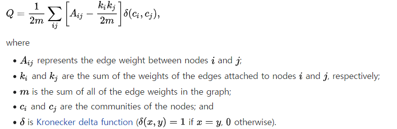
Reference: https://en.wikipedia.org/wiki/Louvain_method

The above equation can be interpreted as the gap between actual edges between clusters and expected edges between clusters for a random graph with the same number of links.

https://en.wikipedia.org/wiki/Louvain_method

• Louvain Community Detection

https://mons1220.tistory.com/129

Since we now have a criterion for a community detection task, we can a conduct community detection task by optimizing this criterion. However, optimizing modularity is an NP-Hard task. Louvain Community Detection is a heuristic that aims to optimize modularity.

Louvain algorithm is a bottom-up greedy algorithm. It means that it starts from one node, and enlarges the cluster by adding a relevant node. Louvain algorithm first assigns each node a different cluster, and then uses an iterative greedy method, repeating 2 steps: 1. local moving of nodes, and 2. Aggregation of the network.

1. Local moving of nodes
   • For each node, we change its cluster into the nearby cluster. Then, if modularity increases, we accept this change. Otherwise, we cancel this change. We conduct this process for every node, until modularity reaches to local optima.
2. Aggregation of the network
   • For the resulting clusters in 1, we consider each cluster as a node, and edges inside the cluster as a self-loop. Then, we obtain a new network, each node being the clusters. Then, with this aggregated network, we move on to 1 again, and then 2, and on and on until there is no change in step 1.

Louvain algorithm is a powerful algorithm due to its speed and easy implementation. Meanwhile, it requires a lot of memory space. Also, while the order of nodes to perform step 1 does not change the final clusters, it does change the speed of the algorithm. For more details, we refer to the original paper.

For other criteria and other algorithms, we refer to https://towardsdatascience.com/community-detection-algorithms-9bd8951e7dae

Deep model based Community Detection: ModNet

While Louvain algorithm is a powerful algorithm, there are attempts to solve modularity optimization problem using deep models. Recently, ModNet showed strong performance. We briefly introduce this method.

The problem with directly applying modularity as a loss function for ML is that this loss is not differentiable. Therefore, the paper uses a soft modularity , which is differentiable, as a loss function.

Here, is an adjacency matrix, is a matrix of probabilities of nodes attribution to clusters ( is a number of nodes and is a hyperparameter denoting the number of communities), and , where is a node degree vector.

The reason the above is "soft" modularity is that it is derived from the natural relaxation of the original modularity formula. We can modify the above modularity formula as follows:

This is just a decomposition of the Kronecker delta into possible cases, . Then, we can generalize and as a probability of containing in certain communities, and . This relaxation results in the formula below, with denotes a probability vector.

It is known that the above two formula for soft modularity coincide. We omit this detail.

Now, we can use this differentiable modularity loss as a loss function for the unsupervised community detection task. However, this soft modularity might have multiple local optima. Therefore, the paper suggests to append the regularizer . They claim this regularizer leads to the solution with similar community size from Symmetric Stochastic Block Model (SSBM), a graph generative model which tends to create a uniform distribution of communities.

Lastly, the model divides the cases into two cases, based on theories in the SSBM model. An associative case is when we can well-perform the community detection, where the number of communities is sufficiently large and each community is distinguishable. A disassociative case is an opposite. Whether each community is distinguishable is determined by the value of Signal-To-Noise Ratio (SNR). We omit the explanation regarding SNR, since it requires a background in SSBM. We can distinguish whether the case is associative or not before we conduct the model, since the number of communities is a hyperparameter and the parameters for SNR are obtained from the raw input graph.

First, The final loss function would be if the case is associative, and . It is because the disassociative case often struggles with negative modularity.

After determining the loss function, we can use deep models to optimize the loss function and solve the community detection task. The choice of network is widely open, including GNN architectures like GCN. However, the most well-performing algorithm was regarding graph data like a NLP data, and use embedding and attention network like NLP task. (Although they did not tried to directly use GAT architecture.) The resulting performance overwhelmed most of both classical and other deep model algorithms, including even supervised methods.

5. Remaining challenges in applying deep model based algorithms to GraphDB

As discussed above, deep models on a graph can handle graph data with efficient implementation and capture its information in a data-driven way instead of pre-determined rules. However, several obstacles still exist when using deep models in GraphDBs.

📌 Memory efficiency

To use a deep models in a GraphDB, it should keep 1) a neural network for graph input or 2) an embedding for graph data. Either way, we need extra memory spaces to hold those data. 1) requires both memory complexity for NN and time-complexity to actually process the data through NN. 2) can save time cost for generating the embedding, but requires more memory space than 1).

📌 Dynamic graph embedding

GraphDBs should be able to handle frequent insertions and deletions of nodes and edges. This implies that our embedding or NN needs to handle dynamic graphs, hopefully in real-time. Many current deep models on a graph mainly focus on static graphs instead of a dynamic graph since learning representations for a dynamic graph is not an easy task. Still, there are some attempts to implement deep models in dynamic graphs.

A dynamic graph can be represented as an ordered list or an asynchronous stream of timed events, such as additions or deletions of nodes and edges. Representing a dynamic graph for a GraphDB is even more complicated since, in addition to the previous streams of timed events, we have also real-time streams. Here we will consider the dynamic graphs with the stream of timed events. Handling real-time streams is an active topic of research.

Here we review DyRep, the representation learning algorithm for dynamic graphs. We review the brief key ideas of the papers and omit details.

For other algorithms, we refer http://web.cs.ucla.edu/~patricia.xiao/files/Paper_Reading_Group_20201006.pdf.

The complicated methods to embed dynamic information shows that there are still many challenges to implementing dynamic graph embedding, even if it is not real-time. We believe researches in this area would play a pivotal role when implementing deep models in a GraphDB.

Dynamic Graph Embedding using a deep model: DyRep

DyRep proposes a method that can handle additions of nodes for an undirected unweighted graph. Note that it does not handle the deletion. DyRep is a complicated algorithm, which shows how hard it is to encode the information of a dynamic graph.

First, We define two types of "event" that change the graph:

• a communication that is temporal, and
• an association that is permanent.

Note that they are not exclusive. For example, when you think of a friendship graph, meeting a new person once is a communication. After the meeting, you might become a permanent friend with the person, which is an association. Or, you might decide not to be friend with the person, which does not lead to the association. An event is defined as a tuple where are nodes, is a time, and is an event type indicator, where 0 stands for association and 1 stands for communication.

Instead of training node representation , the model focuses on learning the representation function of time . When embedding a dynamic graph, the model needs to capture the effect of an event. The algorithm analyzes the effect of the event by decomposing to three messages: Self-propagation, Exogeneuous Drive, and Localized Embedding Propagation. We illustrate this part with the case when event occurs. We denote the a time point right before the current time , and as a time point of the last event on before .

1. Self-Propagation is how the previous embedding of the given node evolves as the new event occurs. It is written by the linear transform of the 's representation at the last time the node got a direct event. Note that it is not the last event of the "graph", but of the "given node". we can write the message from this as
2. Exogenous Drive is how much exogenous effects occur during the exogenous time, the time from the last time directly effected to the current event time. Exogenous time would be and the message is measured by linear transform of exogenous time, .
3. Localized Embedding Propagation is the part we calculate the direct effect of the event, from . First, we aggregate the neighborhood information of and propagate it to . We write it as . Then, we can compute the message by linear transform: .
   • How to aggregate the neighborhood information and construct is a key problem. The authors propose "Temporal Point Process based Attention Mechanism", a modified version of GAT, to do this. The idea is to use both an adjacency matrix, which shows associations, and a stochastic strength matrix, which shows temporal relations that can potentially influence associations. For the time , they are denoted by and .
   • and also need to be evolved dynamically, as an event occurs. The update procedures for the event is described below:
     1. is updated if and only if (association). We update by in this case, and do not update otherwise.
     2. Updating requires branches.
        • If the event is a communication (), and there was an association previously ()
          • We define , the background attention of the graph for the given node . It is a weight and initialized by the uniform distribution of . If the event occurs, we update by , which is done by adding intensity function that will be obtained below. We plug in new into , and do the same update for .
        • If the event is association ()
          • We use same as above and follow the same updates. But in this case, there was a change in a neighborhood of , so we need to adjust the background attention by , where is a neighbors of besides . Then, as we did in the above, we plug-in this value to .
        • Otherwise
          • In this case, we do not need to update .
   • Then with , The model make the attention coefficient of as . We then construct by and .

• Now, we aggregate these three messages to calculate the total message of the given event. The paper uses "sum" as a function.
• Lastly, we update the representation using the function. The paper uses the activation function as a update function. .