1. Introduction

Recently, research on the geometric properties of value functions and attempts to apply these properties to various fields of Reinforcement Learning (RL) have been actively conducted. This post is an introduction to Value Function Geometry including an introduction of the paper "The Value Function Polytope in Reinforcement Learning" by Dadashi et al 1.

This post aims to explain the basic concepts of value function linear approximation and representation learning. Also, the paper 1 establishes the geometric shape of value function space in finite state-action Markov decision processes: a general polytope. By reimplementing the paper myself, I was able to check the surprising theorems and geometric properties. I have attached some results that I checked directly in the post.

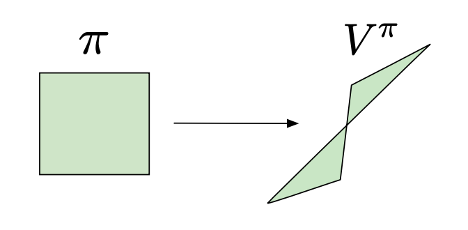
Figure 1: Mapping between policies and value functions 1

2. Background

We usually consider an environment with a Markov Decision Process(MDP) in Reinforcement Learning 2. Markov Decision Process is a Markov reward process with decisions, where is the state space, is the action space, is the reward function, is the transition function, and (0,1) is the discount factor.

A stationary policy is a mapping from states to distributions over actions . We denote the space of all policies by . Given a policy and a transition function , we can obtain the state-to-state transition function

State-value function

The return is the total discounted reward from time-step and state by following a policy ; and are the state and action at time .

The state-value function is defined as the expected return starting from a particular state and following policy .

Action-value function

The action-value function is defined as the expected return starting from a particular state and action, and then following policy .

In particular, the state-value function is an expectation over the action-value functions under a policy .

In the case, we take an action by following an argmax policy ,

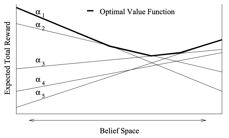
Figure 2: Geometric View of Value Function 3

Figure 2 represents the geometric relationship between the state-value function and the action-value function, when following an argmax policy. Each line corresponds to the action-value function and the bold line corresponds to the state-value function. It can be seen that the maximum action-value selected for each state is the state-value function. In Figure 2, it can also be checked that does not play any useful role in the state-value function.

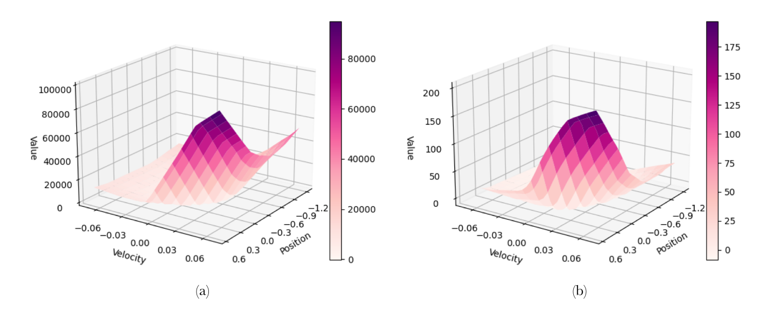
Figure 3: Value Functions for the mountain car problem using DQN

Figure 3 is an example of value functions that I obtained for the mountain car problem. Both used DQN (Deep Q-Networks) to train the agent. Figure 3(a) is based on 2000 runs of mountain car without changing the reward, and Figure 3(b) is based on 500 runs of mountain car with adding a heuristic reward. I gave a bonus reward of 15 times the velocity of the next state. By giving a heuristic reward to the agent, the mountain car was able to learn and train faster.

3. Value Function Linear Approximations

A value function for a policy is denoted as , and a d-dimensional representation is a mapping ; is the feature vector for state , where are the feature functions.

For a given representation with a weight vector , the linear approximation for a value function is defined as:

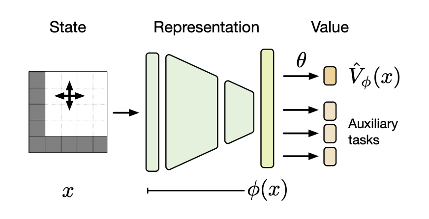
Figure 4: A deep reinforcement learning architecture viewed as a two-part approximation 4

Bellman operator

Assume a finite state space:

Let's start by introducing some vector and matrix notation to make it more convenient.

It is well known that the state-value function satisfies Bellman's equation:

Given a policy , we define the Bellman operator as:

Since satisfies Bellman's equation, is the fixed point of operator ; . Then,

In the case, we do not know the entire model completely, we cannot calculate explicitly by the above equation. However, by starting with any vector and applying the Bellman operator repeatedly, it will finally converge and reach the fixed point . This can be explained by the Contraction Mapping Theorem.

Projection operator

Projection operator is a widely used operator in Statistics for Multiple Linear Regression Models and Least Squares Estimation.

For an matrix of full column rank, is the column space of , the linear subspace in spanned by the columns of the matrix .

We let denote the projection operator for subspace spanned by such that

Projector operator satifies the normal equations:

What if is not invertible? Then, we will have infinite solutions for and . However, since is full column rank, it implies that is positive definite and invertible.

Back to the value function approximation, let's assume a finite state space of states; . Also, we write to denote the matrix whose columns are .

We consider the approximation minimizing the squared error:

performs an orthogonal projection of value function vector onto the linear subspace . So, is the value function we seek when doing linear function approximation in subspace defined by minimizing .

4. Value Function Polytope in Reinforcement Learning

Definition 1 : Polytope

is a convex polytope in iff there are points such that .

We write to denote the convex hull of the points .

is a (possibly non-convex) polytope iff it is a finite union of convex polytopes.

Definition 2 : Polyhedron

is a convex polyhedron iff there are half-spaces
whose intersection is , that is

is a (possibly non-convex) polyhedron iff it is a finite union of convex polyhedra.

The Space of Value Functions

The main contribution of Dadashi et al 1 is the characterization of the space of value functions. The space of value functions is the set of all value functions obtained from all possible policies.

Dadashi et al 1 show that is a polytope. Instead of proving it directly by the definition of (convex) polytope, they use the important proposition that a bounded, convex polyhedron is a convex polytope 6.

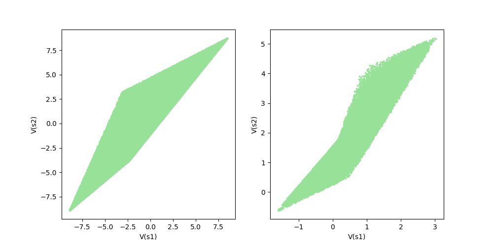
Figure 5: Space of Value Functions for 2-state MDPs

Figure 5 depicts the value function space corresponidng to two different 2-state MDPs. The space is made of 100,000 value functions corresponding to 100,000 randomly sampled policies from . The specific details of MDPs presented in this figure are as follows.

Figure 5: Left

Figure 5: Right

I used the following convention to express , (also the paper):

To easily check the shape of the polytope, I checked with the value function spaces from 2-state MDPs, which is convenient to visualize. The policy space is the Cartesian product of simplices. However, in general, a wide variety of polytope shapes are possible for the value function space .

In fact, if you look closely at the right of Figure 5, you'll find something a little odd. You may think it's not a perfect polytope because the upper left hand is a little empty. To double-check if the policy was sampled uniformly from the policy space, I visualized the mapping between policy samples and value function samples.

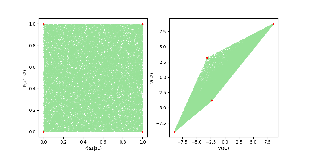
Figure 6: Mapping between sample policies and sample value functions. The red points are the value functions of deterministic policies

To easily visualize the policy space and value function space, 2-state 2-action MDP was used for Figure 6. It includes 50,000 pairs of policy and value function samples. The specific details of MDP presented in this figure are as follows.

The left of Figure 6 definitely shows that the policy has been sampled uniformly. Despite the uniformly selected policies, you can still see the sparse empty space in the upper left corner of the value function space. Also, to confirm the existence of the polytope's vertex, I took the value functions of deterministic policies and confirmed that they become the vertex. In conclusion, we can know that the sparse empty space in the figure is simply due to the lack of sample numbers. It can also be seen that the polytope of the value function space does not consist of equal density.

Definition 3 : Policy Agreement

Two policies agree on states if for each

For a given policy , we will denote by the set of policies which agree with on . Thus, , for , describes the set of policies that agree with on all states except .

Definition 4 : Policy Determinism

A policy is

• -deterministic for if .
• semi-deterministic if it is -deterministic for at least one .
• deterministic if it is -deterministic for all states .

We denote by the set of semi-deterministic policies that take action on state .

Value Functions and Policy Agreement

Now, I will introduce one of the most amazing theorem of this paper, line theorem. It characterizes the subsets of value function space that are generated by the policies which agree on all but one state. Surprisingly, it describes a line segment within the value function polytope and this line segment is monotone.

Theorem 1 : Line Theorem

Let be a state and , a policy. Then there are two -deterministic policies in , denoted , which bracket the value of all other policies

Furthermore, the image of restricted to is a line segment, and the following three sets are equivalent:

Furthermore, the image of restricted to is a line segment, and the following three sets are equivalent:

Theorem 1 implies that we can generate , the image of restricted to , by drawing the value functions of mixtures of two policies, and . Also, we can even generate it by just taking two value functions, and , and drawing a line segment between the two points.

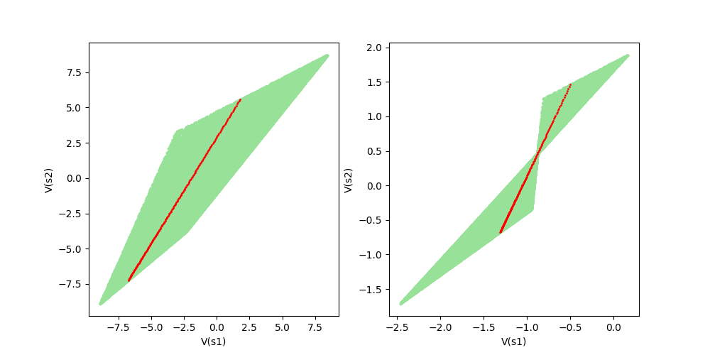
Figure 7: Illustration of Theorem 1 Line Theorem.

Figure 7 actually illustrates the value function space drawn by the interpolated policies between and . The red points describe the value functions of mixtures of policies that agree everywhere but one state. By sampling 200 mixtures of policies that agree but one state and drawing each value function, we could see it forms a line segment. The specific details of MDPs presented in Figure 7 are as follows.

Figure 7: Left

Figure 7: Right

For both figures in Figure 7, the following and which agree on were used for the interpolation.

where .

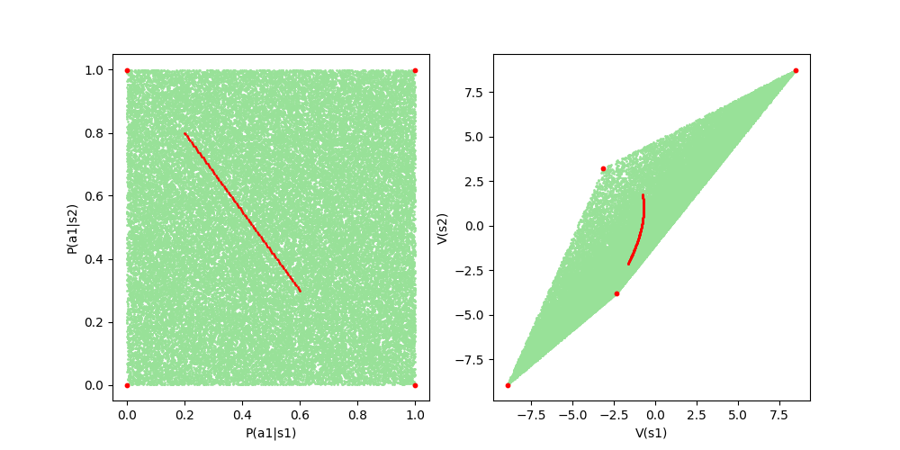
Figure 8: Value functions of mixtures of two policies in the general case.

The red points in Figure 8 are the value functions of mixtures of two policies. You can see that the red points are curved, not straight. It can be seen that the condition, the policies should agree on all but one state, is a necessary condition.

By visualizing the policy space, we can easily recognize that the two policies do not agree on any states. In the case of and , if the two policies agree on one state, the interpolation of the two policies shall be horizontal or vertical. The specific details of MDP presented in Figure 8 are same as the MDP presented in Figure 7: Left, and following and were used for mixtures.

Corollary 1.* *For any set of states and a policy , can be expressed as a convex combination of value functions of -deterministic policies. In particular, is included in the convex hull of the value functions of deterministic policies.

Corollary 1 can be proved by mathematical induction on the number of states . The result of are seen directly from the Line Theorem.

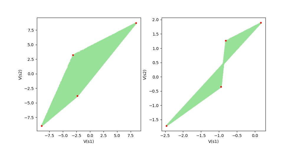
Figure 9: Visual representation of Corollary 1. The red dots are the value functions of deterministic policies.

As you can see in Figure 9, the space of value functions is included in the convex hull of value functions of deterministic policies. Also, you can check the relationship between the vertices of and deterministic policies. However, in Figure 10, we can also observe the fact that the value functions of deterministic policies are not necessarily the vertices of and that the vertices of are not necessarily the value functions of deterministic policies.

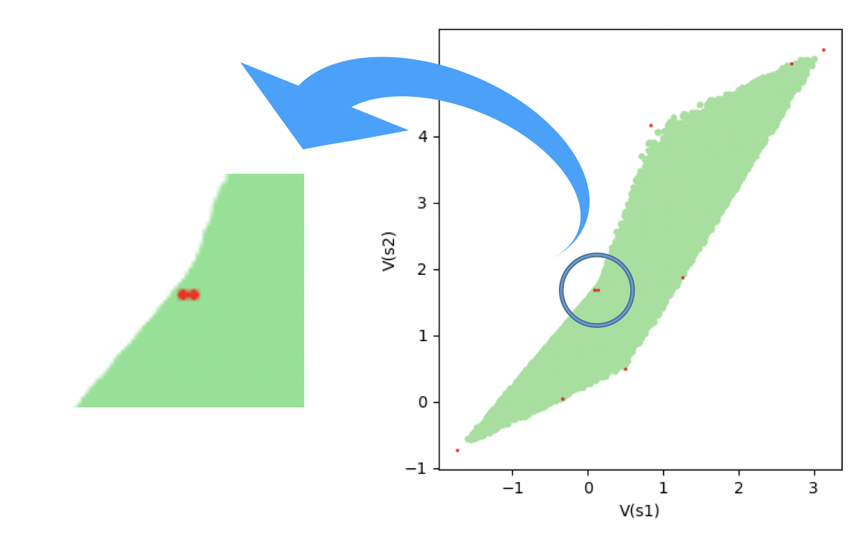
Figure 10: Visual representation of Corollary 1. The value functions of deterministic policies are not identical to the vertices of V.

The Boundary of

Theorem 2 and Corollary 3 show that the boundary of value function space is described by semi-deterministic policies.

Let's start with first defining the affine vector space before we mention Theorem 2. Consider a policy and states . Then,

where are the columns of the matrix corresponding to states other than .

Theorem 2.

Consider the ensemble of policies that agree with on states . Suppose , , s.t. , then has a relative neighborhood in .

Corollary 3.* *Consider a policy , the states , and the ensemble of policies that agree with on . Define , we have that the relative boundary of in is included in the value functions spanned by policies in that are s-deterministic for

where refers to the relative boundary .

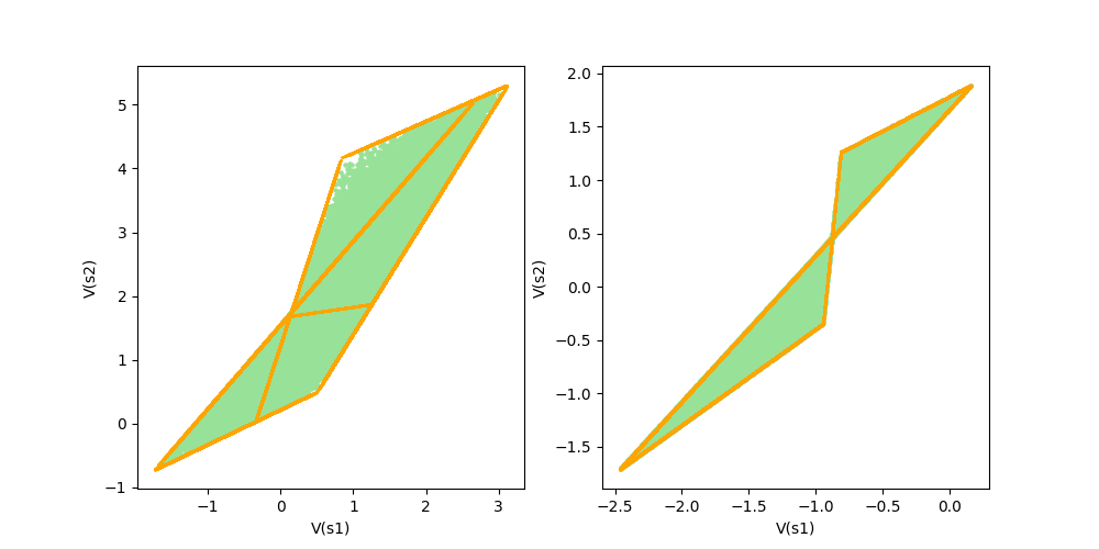
Figure 11: Visual representation of Corollary 3. The orange points are the value functions of semi-deterministic policies.

The Polytope of Value Functions

By combining all the previous results, Dadashi et al 1 proved the value function space is a polytope. Theorem 3 is the final result of this paper 1.

Theorem 3.

Consider a policy , the states , and the ensemble of policies that agree with on . Then is a polytope and in particular, is a polytope.

Theorem 3 can be proved by induction on , the cardinality of the number of states. If , is the set of policies which agree with on every state. Since only can agree with on every state, . Therefore, is a polytope. Now, assume the theorem is true for and prove that it is true for . This will prove the Theorem 3.

5. Summary

There have been many developments in the field of value function geometry recently. In the case of finite state-action spaces, Dadashi et al 1 characterized the shape of value function space: a general polytope. It helps our understanding of the dynamics of reinforcement learning algorithms.

Although there is still a problem with generalizing to infinite or continuous state-action spaces, it is certain to be a great study that has created a new direction exploring the field of reinforcement learning. Bellemare et al 4 discovered a connection between representation learning and the polytopal structure of value functions, and a number of follow-up papers are being published 7 8. Also, exploring the relationship between value function approximation and the geometry of value functions will be another interesting field of study.

Before joining ML2, I did not have a good understanding of reinforcement learning. However, thanks to all of the members of ML2, I was able to gain valuable research experience in reinforcement learning and the field of value function geometry during my internship. I am still deeply interested in developing the research during my internship.

Reference

1

Dadashi, R., Taiga, A. A., Roux, N.L., Schuurmans, D., and Bellemare, M. G.
The value function polytope in reinforcement learning, In ICML, 2019.

2

Sutton, R. S. and Barto, A. G.
Reinforcement Learning: An Introduction, MIT Press, 2nd edition, 2018.

3

Poupart, P. and Boutilier, C.
Value-Directed Belief State Approximation for POMDPs,arXiv preprint arXiv:1301.3887, 2013.

4

Bellemare, M. G., Dabney, W., Dadashi, R., Taiga, A. A., Castro, P. S., Roux, N. L., Schuurmans, D., Lattimore, T., and Lyle, C.
A geometric perspective on optimal representations for reinforcement learning, In Neural Information Processing Systems (NeurIPS), 2019.

5

Rao, A.
Value Function Geometry and Gradient TD, Stanford CME 241 Lecture Slides, 2020.

6

Ziegler, G. M.
Lectures on Polytopes, volume 152. Springer Science & Business Media, 2012.

7

Dabney, W., Barreto, A., Rowland, M., Dadashi, R., Quan, J., Bellemare, M. G. and Silver, D.
The Value-Improvement Path Towards Better Representations for Reinforcement Learning, arXiv preprint arXiv:2006.02243, 2020.

8

Ghosh, D. and Bellemare, M. G.
Representations for Stable Off-Policy Reinforcement Learning, arXiv preprint arXiv:2007.05520, 2020.