Preface

Reinforcement Learning (RL) has become one of the major categories in the field of machine learning in the recent years via the breakthroughs such as approximation of complex non-linear function through deep neural networks. Among these, a distributional perspective on the value function estimation has contributed on taking a big jump in the performance of RL algorithms. However, proper discussions of distributional RL (DRL) are still limited to specific algorithms or network architectures such as Q-learning or deterministic policy gradient.

In the situation at hand, we have worked to address some of the critical aspects in RL that was left out in the distributional perspective. The details and the findings of this journey can be found in our recent work "GMAC: A Distributional Perspective on Actor-Critic Framework" which was published in the International Conference on Machine Learning (ICML), 2021. In this paper, we expand the distributional perspective to actor-critic framework, more specifically for the well known algorithm Proximal Policy Optimization (PPO). Along the way, we discuss the changes that were made to the components of the widely used DRL algorithms and introduce new algorithms to efficiently formulate and learn from the distributional Bellman targets of the estimated state values.

Distributional Reinforcement Learning

Before jumping in, we will briefly review what DRL is, conceptually. Imagine being at some state at time t, and following a stochastic policy in a given MDP. Following this policy for some time will yield a trajectory as shown in the figure below

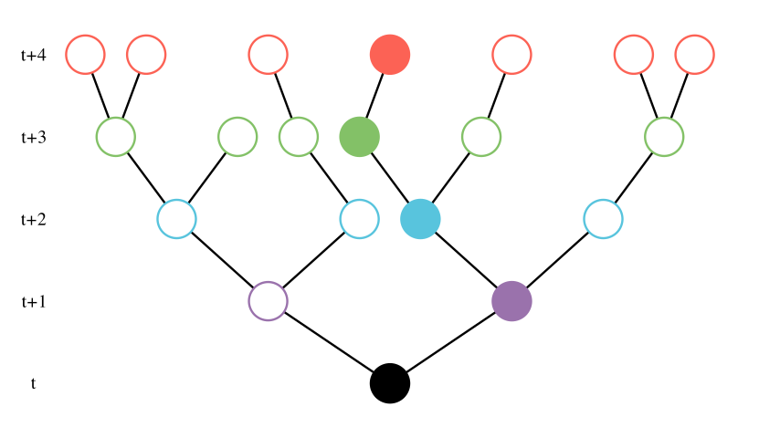
Here, the black node represents the state at time t and consecutive filled nodes are the states of a trajectory generated following . As seen in the figure, only one trajectory was selected but many more trajectories could have been the ones selected from the stochasticity of the policy and state transitions. If we can capture those stochasticity and represent them through a distribution, we may be able to gain a better insight on the outcomes and consequences of following some policy at a given state, leading to more informed evaluation of a state compared to scalar expectation.

The origin of distributional modeling of the state value dates quite back, even to the late 70's. However, in the context of modern deep RL, the terminology "distributional RL" usually refers to a perspective worked out by Bellemare et al. in the paper "A Distributional Perspective to Reinforcement Learning" (ICML, 2017). Briefly speaking, DRL estimates a distribution over possible values given a state instead of the traditional expectation of the of the value. Bellemare et al. builds the foundation of this framework on the Wasserstein metric and proves that the distribution converges just as in the original scalar version of learning by Bellman equation. But other than simply showing that it works, there has to be a reason on why we should make it work.

Learning the distribution of the values reveals to us much more information that may help making decisions compared to having access only to the expectation. Consider the following figure:

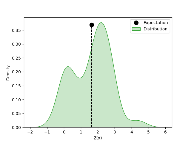
In this figure, the scalar value of the expectation has little information about what may happen in the future while the whole distribution tells about information like variance, modes, symmetricity, and so on. These information may become useful when estimating the risk, confidence, and comparing actions and states with same expectations. For example in the following figure,

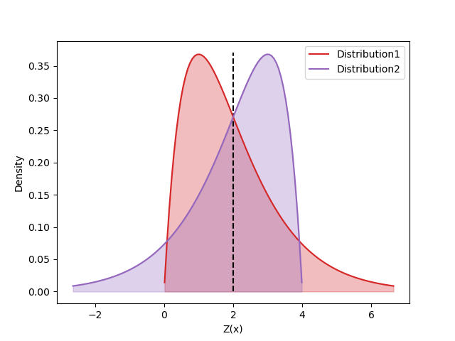
the distributions in each graph have same expectations but their skewness are in the exact opposite direction of each other.

Data conflation and Cramér Distance

So far, we have discussed the advantages that a distributional perspective can bring on RL. Here we present more technical details on how the learning of value distribution can be put to a practical method.

Quick Overview

In the distributional perspective of RL, the value distributions, are described by the distributional Bellman equation which states

where is the reward distribution and is the discount factor. Then, within the Wasserstein metric space, the distributional Bellman operator, is a contraction mapping. Thus theoretically, we can successfully find a unique, stationary solution using the distributional Bellman operation.

In practical sense, roughly there are two branches of works suggesting the methods to perform the Bellman update between and .

• Minimize cross-entropy between the two bounded discrete distributions in C51.
• Minimize Huber-quantile loss between random samples of the two distributions in QR-DQN.

The first was suggested in Bellemare et al. (2017) and the second was suggested in Dabney et al. (2018). The Wasserstein distance is biased in a sample gradient and instead turns to minimizing the cross-entropy of the Kullback-Leibler divergence between and projected onto the support of . The QR-DQN suggests a method to bridge this theory-practice gap of moving away from minimizing the Wasserstein distance: parametrizing the quantiles and minimizing the Wasserstein distance through quantile-regression.

On the other hand, because quantile-regression is non-differentiable at 0, Huber-quantile, a smooth version of the quantile-regression was used instead. This however had a problem known as data conflation (Rowland et al. 2019) which results with underestimation of variance of the modeled distribution when multiple Bellman operations were applied.

Cramér distance

Underestimation of variance quickly becomes more problematic for actor-critic method since many well-known actor critic methods are on-policy learning, meaning they will learn from longer horizon compared to the off-policy methods. For example, PPO (Proximal Policy Optimization, Schulman et al. 2016) collects trajectories of length 128 for Atari games. This means that there are samples in GAE (General Advantage Estimate) that will have had 128 Bellman operations applied, and the data conflation now becomes critical. To solve this issue, we turn to a different loss function that will not suffer from the data conflation.

The Cramér- distance, which we choose as the base of the distance function, is defined as

where and are random variables and is the c.d.f. of the subscripted random variable. When , the Cramér distance is also equivalent to the energy distance defined as

Similarly, the distributional Bellman operator is also a -contraction mapping in Energy distance metric. In summary, we propose to use minimize the energy distance between the distribution estimation and the distributional Bellman target.

Achieving efficiency through SR()

So far, we have discussed what distance function we will be using. Here, we discuss how the Bellman target can be formed efficiently. If we intend to use n-step return distributions as the Bellman target distribution, the complexity of calculating that distribution would just be same as in the scalar version. The problem occurs when we want to mix different n-step returns as in TD(). Assuming that we have empirical distribution for each state in the trajectory, producing an empirical distribution of the mixture of different n-step return for all states in the trajectory can be achieved in linear complexity using our proposed algorithm called SR() (sample-replacement-lambda). The whole process of the algorithm is graphically depicted in the video below.

Performance improvement using Gaussian Mixture Model

The performance of suggested method was tested in the Atari 2600 tasks. Using PPO as the backbone, the SR() enabled efficient generation of distributional Bellman targets analogous to the TD(). Then, minimizing the Cramér distance actually improved the performance over that of the scalar version of PPO. Taking a step further, we suggest to parameterize the predicted distribution using Gaussian mixture model (GMM). Using GMM, the random variable is defined as

When using the GMM, the analytic solution to energy distance between GMM can be found and the SR() can be performed on pair instead of a sample to pass on more information like variance in compared to a single sample. When GMM was applied, the performance improved even more significantly as seen in the figure below.

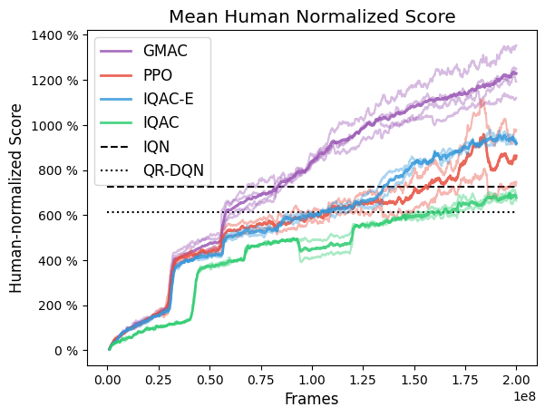
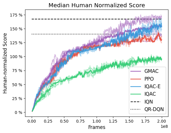
In the figure, the red labeled PPO is the original scalar version of PPO. Changing its value estimation to quantiles and using Huber-quantile as in IQN yields the green plot labeled IQAC. From there, changing the distance function to the energy distance yields the blue plot labeled IQAC-E. Finally, even changing the parameterization of the value function to GMM yields purple plot labeled GMAC.

Further discussion

Throughout this blog, we have covered some of the intuitions behind the development of our recent paper GMAC. So what can we do with distributional algorithms that a scalar version could not do? The paper itself does not directly answer this questions but we give a naive example to illustrate a possible application. Take for example the following two distributions.

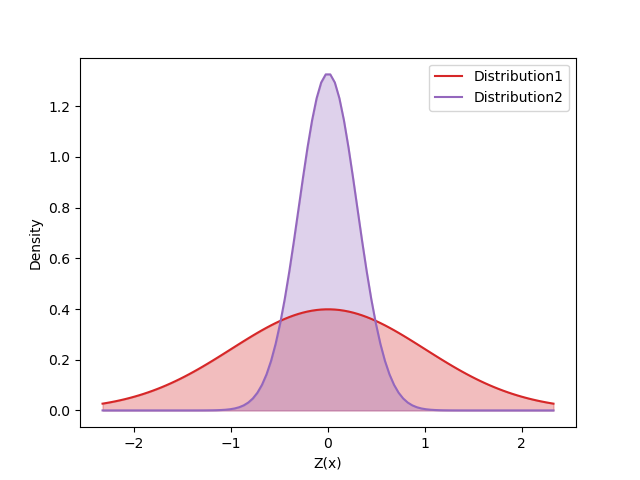
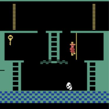
Both distributions have expectation of zero meaning that there has not been any useful reward signal from the environment. To be more precise, let us assume that the environment has only output zero reward for all states so far in the training. Just by observing their expectations, the two distributions are identical. However, the variances let us clearly distinguish the two and suggest that the purple distribution may be closer to the terminal state or have been updated (visited) more. These types of scenarios can be often found in sparse reward hard exploration tasks like Montezuma's Revenge.

Building on this idea, we imagine cases where agent assigns more credit to novel states. A possible way to tell if a state is novel is to observe its Bellman error, as states that have been visited frequently would have been updated more and thus its Bellman error is expected to be less. However, using the popular technique, the network is initialized to output values very close to zero, leading to Bellman errors of zero for nearly all states to start with. On the other hand, when the model is parameterized as GMM, the initialization leads to output of standard normal very close to standard normal at the beginning. In this case, the states that have been visited would have very low variance relative to the novel states and thus using the divergence metric such as the energy distance as an intrinsic motivation enables the agent to better explore. A result of actual experimentation on this concept is shown in the following figure:

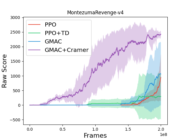
Here, using GMAC with the intrinsic motivation achieves a significant improvement in Montezuma's revenge compared to the version without the intrinsic motivation or the scalar version which uses the TD-error as the motivation. This result clearly hints us on how distributional RL can tackle other tasks that scalar version may struggle with.

We kindly invite the curious readers who wish to peek into more details on this subject to the actual paper.

References

1.

Bellemare, M. G., Dabney, W., and Munos, R. A dis- tributional perspective on reinforcement learning. In Proceedings of the 34th International Conference on Machine Learning ICML, 2017.

2.

Dabney, W., Rowland, M., Bellemare, M. G., and Munos, R. Distributional reinforcement learning with quantile regression. In AAAI, pp. 2892–2901, 2018.

3.

Rowland, M., Dadashi, R., Kumar, S., Munos, R., Belle- mare, M. G., and Dabney, W. Statistics and samples in distributional reinforcement learning. In Chaudhuri, K. and Salakhutdinov, R. (eds.), Proceedings of the 36th International Conference on Machine Learning ICML, 2019.